Lanczos algorithm

The Lanczos algorithm is an iterative algorithm invented by Cornelius Lanczos that is an adaptation of power methods to find eigenvalues and eigenvectors of a square matrix or the singular value decomposition of a rectangular matrix. It is particularly useful for finding decompositions of very large sparse matrices. In latent semantic indexing, for instance, matrices relating millions of documents to hundreds of thousands of terms must be reduced to singular-value form.

1 Power method for finding eigenvalues
2 Lanczos method
- 2.1 The algorithm
- 2.2 Numerical stability
3 Variations
- 3.1 Nullspace over a finite field
4 Applications
5 References
6 External links

Power method for finding eigenvalues

The power method for finding the largest eigenvalue of a matrix $A\,$ can be summarized by noting that if $x_0\,$ is a random vector and $x_{n%2B1} = A x_n\,$ , then in the large $n$ limit, $x_n/||x_n||$ approaches the normed eigenvector corresponding to the largest eigenvalue.

If $A = U \operatorname{diag}(\sigma_i) U' \,$ is the eigenvalue decomposition of $A\,$ , then $A^n = U \operatorname{diag}(\sigma_i^n) U'$ . As $n\,$ gets very large, the diagonal matrix of eigenvalues will be dominated by whichever eigenvalue is largest (neglecting the case where there are large equal eigenvalues, of course). As this happens, $|x_{n%2B1}| / |x_{n}|\,$ will converge to the largest eigenvalue and $x_n / |x_n|\,$ to the associated eigenvector. If the largest eigenvalue is multiple, then $x_n \,$ will converge to a vector in the subspace spanned by the eigenvectors associated with those largest eigenvalues. After you get the first eigenvector/value, you can successively restrict the algorithm to the null space of the known eigenvectors to get the other eigenvector/values.

In practice, this simple algorithm does not work very well for computing very many of the eigenvectors because any round-off error will tend to introduce slight components of the more significant eigenvectors back into the computation, degrading the accuracy of the computation. Pure power methods also can converge slowly, even for the first eigenvector.

Lanczos method

During the procedure of applying the power method, while getting the ultimate eigenvector $A^{n-1} v$ , we also got a series of vectors $A^j v, \, j=0,1,\cdots,n-2$ which were eventually discarded. As $n$ is often taken to be quite large, this can result in a large amount of disregarded information. More advanced algorithms, such as Arnoldi's algorithm and the Lanczos algorithm, save this information and use the Gram–Schmidt process or Householder algorithm to reorthogonalize them into a basis spanning the Krylov subspace corresponding to the matrix $A$ .

The algorithm

The Lanczos algorithm can be viewed as a simplified Arnoldi's algorithm in that it applies to Hermitian matrices. The $m$ 'th step of the algorithm transforms the matrix $A$ into a tridiagonal matrix $T_{mm}$ ; when $m$ is equal to the dimension of $A$ , $T_{mm}$ is similar to $A$ .

Definitions

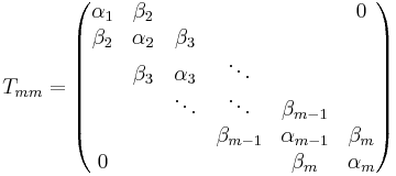
We hope to calculate the tridiagonal and symmetric matrix $T_{mm} = V_m^* A V_m.$

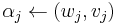
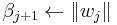
The diagonal elements are denoted by $\alpha_j = t_{jj}$ , and the off-diagonal elements are denoted by $\beta_j = t_{j-1,j}$ .

Note that $t_{j-1,j} = t_{j,j-1}$ , due to its symmetry.

Iteration

(Note: Following these steps alone will not give you the correct eigenvalue and eigenvectors. More consideration must be applied to correct for the numerical errors. See the section Numerical stability in the following.)

There are in principle four ways to write the iteration procedure. Paige[1972] and other works show that the following procedure is the most numerically stable.^[1]^[2]

Algorithm Lanczos
  random vector with norm 1.
 
 
 Iteration: for 
     
     
     
     
     
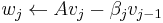
 return

"←" is a loose shorthand for "changes to". For instance, "largest ← item" means that the value of largest changes to the value of item.
"return" terminates the algorithm and outputs the value that follows.

Note that (x,y) represents the dot product of vectors x and y here.

After the iteration, we get the $\alpha_j$ and $\beta_j$ which constructs a tridiagonal matrix

$T_{mm} = \begin{pmatrix} \alpha_1 & \beta_2 & & & & 0 \\ \beta_2 & \alpha_2 & \beta_3 & & & \\ & \beta_3 & \alpha_3 & \ddots & & \\ & & \ddots & \ddots & \beta_{m-1} & \\ & & & \beta_{m-1} & \alpha_{m-1} & \beta_m \\ 0 & & & & \beta_m & \alpha_m \\ \end{pmatrix}$

The vectors $v_j$ (Lanczos vectors) generated on the fly constructs the transformation matrix

$V_m = \left( v_1, v_2, \cdots, v_m \right)$ ,

which is useful for calculating the eigenvectors (see below). In practice, it could be saved after generation (but takes a lot of memory), or could be regenerated when needed, as long as one keeps the first vector $v_1$ . At each iteration the algorithm executes a matrix-vector multiplication and 7n further ﬂoating point operations.

Solve for eigenvalues and eigenvectors

After the matrix $T_{mm}$ is calculated, one can solve its eigenvalues $\lambda_i^{(m)}$ and their corresponding eigenvectors $u_i^{(m)}$ (for example, using the QR algorithm or Multiple Relatively Robust Representations (MRRR)). The eigenvalues and eigenvectors of $T$ can be obtained in as little as $\mathcal{O}(m^2)$ work with MRRR; obtaining just the eigenvalues is much simpler and can be done in $\mathcal{O}(m^2)$ work with spectral bisection.

It can be proved that the eigenvalues are approximate eigenvalues of the original matrix $A$ .

The Ritz eigenvectors $y_i$ of $A$ can be calculated by $y_i = V_m u_i^{(m)}$ , where $V_m$ is the transformation matrix whose column vectors are $v_1, v_2, \cdots, v_m$ .

Numerical stability

Stability means how much the algorithm will be affected (i.e. will it produce the approximate result close to the original one) if there are small numerical errors introduced and accumulated. Numerical stability is the central criterion for judging the usefulness of implementing an algorithm on a computer with roundoff.

For the Lanczos algorithm, it can be proved that with exact arithmetic, the set of vectors $v_1, v_2, \cdots, v_{m%2B1}$ constructs an orthogonal basis, and the eigenvalues/vectors solved are good approximations to those of the original matrix. However, in practice (as the calculations are performed in floating point arithmetic where inaccuracy is inevitable), the orthogonality is quickly lost and in some cases the new vector could even be linearly dependent on the set that is already constructed. As a result, some of the eigenvalues of the resultant tridiagonal matrix may not be approximations to the original matrix. Therefore, the Lanczos algorithm is not very stable.

Users of this algorithm must be able to find and remove those "spurious" eigenvalues. Practical implementations of the Lanczos algorithm go in three directions to fight this stability issue:

Prevent the loss of orthogonality
Recover the orthogonality after the basis is generated
After the good and "spurious" eigenvalues are all identified, remove the spurious ones.

Variations

Variations on the Lanczos algorithm exist where the vectors involved are tall, narrow matrices instead of vectors and the normalizing constants are small square matrices. These are called "block" Lanczos algorithms and can be much faster on computers with large numbers of registers and long memory-fetch times.

Many implementations of the Lanczos algorithm restart after a certain number of iterations. One of the most influential restarted variations is the implicitly restarted Lanczos method,^[3] which is implemented in ARPACK.^[4] This has led into a number of other restarted variations such as restarted Lanczos bidiagonalization.^[5] Another successful restarted variation is the Thick-Restart Lanczos method,^[6] which has been implemented in a software package called TRLan.^[7]

Nullspace over a finite field

Peter Montgomery published in 1995 an algorithm, based on the Lanczos algorithm, for finding elements of the nullspace of a large sparse matrix over GF(2); since the set of people interested in large sparse matrices over finite fields and the set of people interested in large eigenvalue problems scarcely overlap, this is often also called the block Lanczos algorithm without causing unreasonable confusion. See Block Lanczos algorithm for nullspace of a matrix over a finite field.

Applications

Lanczos algorithms are very attractive because the multiplication by $A\,$ is the only large-scale linear operation. Since weighted-term text retrieval engines implement just this operation, the Lanczos algorithm can be applied efficiently to text documents (see Latent Semantic Indexing). Eigenvectors are also important for large-scale ranking methods such as the HITS algorithm developed by Jon Kleinberg, or the PageRank algorithm used by Google.

References

^ Cullum and Willoughby, Lanczos Algorithms for Large Symmetric Eigenvalue Computations, Vol. 1, ISBN 0-8176-3058-9(v.1)
^ Yousef Saad, Numerical Methods for Large Eigenvalue Problems, ISBN 0-470-21820-7, http://www-users.cs.umn.edu/~saad/books.html
^ D. Calvetti, L. Reichel, and D.C. Sorensen (1994). "An Implicitly Restarted Lanczos Method for Large Symmetric Eigenvalue Problems". ETNA. http://etna.mcs.kent.edu/vol.2.1994/pp1-21.dir/pp1-21.ps.
^ R. B. Lehoucq, D. C. Sorensen, and C. Yang (1998). "ARPACK Users Guide: Solution of Large-Scale Eigenvalue Problems with Implicitly Restarted Arnoldi Methods". SIAM. http://www.ec-securehost.com/SIAM/SE06.html.
^ E. Kokiopoulou and C. Bekas and E. Gallopoulos (2004). "Computing smallest singular triplets with implicitly restarted Lanczos bidiagonalization". Appl. Numer. Math.. doi:10.1016/j.apnum.2003.11.011.
^ Kesheng Wu and Horst Simon (2000). "Thick-Restart Lanczos Method for Large Symmetric Eigenvalue Problems". SIAM. doi:10.1137/S0895479898334605.
^ Kesheng Wu and Horst Simon (2001). "TRLan software package". http://crd.lbl.gov/~kewu/trlan.html.

External links

Golub and van Loan give very good descriptions of the various forms of Lanczos algorithms in their book Matrix Computations
Andrew Ng et al., an analysis of PageRank
Lanczos and conjugate gradient methods B. A. LaMacchia and A. M. Odlyzko, Solving Large Sparse Linear Systems Over Finite Fields
Matlab comes with ARPACK built-in. Both stored and implicit matrices can be analyzed through the eigs() function.
A Matlab implementation of the above algorithm (note precision issues) is available as apart of the Gaussian Belief Propagation Matlab Package.
GraphLab GraphLab collaborative filtering library, large scale parallel implementation of Lanczos (in C++) for multicore.

Numerical linear algebra

Key concepts	Floating point · Numerical stability · BLAS

Problems	Matrix multiplication · Matrix decompositions · Linear equations · Sparse problems

Hardware	CPU cache · TLB · Cache-oblivious algorithm · SIMD · Multiprocessing

Software	Specialized libraries · General purpose software